Q&A 9 How do you visualize RNA-Seq samples using PCA in R?

9.1 Explanation

Principal Component Analysis (PCA) reduces the dimensionality of high-throughput data like RNA-Seq by finding the principal directions of variation. PCA is useful for:

• Detecting sample outliers
• Checking for batch effects
• Visualizing group separation

We apply PCA on the rlog-transformed data (rlog_matrix.csv) to ensure homoscedasticity and interpretability.

9.2 R Code

library(tidyverse)

# 📥 Load rlog-transformed matrix
rlog_mat <- read_csv("data/rlog_matrix.csv")

# 🧪 Prepare PCA input
pca_input <- rlog_mat |>
  column_to_rownames("gene") |>
  t() |>
  as.data.frame()

# 📊 Run PCA
pca_res <- prcomp(pca_input, center = TRUE, scale. = TRUE)
pca_df <- as_tibble(pca_res$x) |>
  mutate(Sample = rownames(pca_input))

# 🔗 Join with metadata
metadata <- read_csv("data/demo_metadata.csv")
plot_df <- left_join(pca_df, metadata, by = "Sample")

# 🎨 Plot
ggplot(plot_df, aes(x = PC1, y = PC2, color = condition)) +
  geom_point(size = 3, alpha = 0.8) +
  labs(title = "PCA of RNA-Seq Samples",
       x = paste0("PC1 (", round(summary(pca_res)$importance[2, 1] * 100, 1), "%)"),
       y = paste0("PC2 (", round(summary(pca_res)$importance[2, 2] * 100, 1), "%)")) +
  theme_minimal()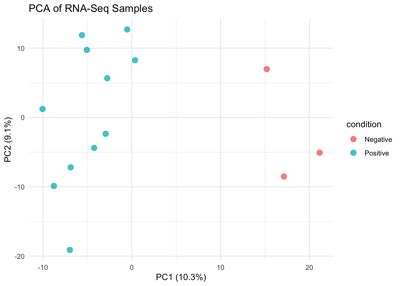

✅ Takeaway: PCA on log-transformed RNA-Seq data helps visualize sample similarities, spot outliers, and confirm that experimental conditions drive the major sources of variation.