counts <- readr::read_csv("data/demo-counts.csv", show_col_types = FALSE)

dim(counts)
[1] 500 13Before modeling, we must confirm that the count matrix is structurally sound.
Errors at this stage propagate silently into downstream analyses.
Quality control at this level focuses on:
counts <- readr::read_csv("data/demo-counts.csv", show_col_types = FALSE)
dim(counts)[1] 500 13The first column should be gene_id.
Remaining columns correspond to samples.
all(sapply(counts[-1], is.numeric))[1] TRUEAll sample columns must be numeric.
Library size is the total number of reads per sample.
library_sizes <- colSums(counts[-1])

library_sizes
sample-01 sample-02 sample-03 sample-04 sample-05 sample-06 sample-07 sample-08
7684 8351 13817 9176 9442 14177 12318 7689
sample-09 sample-10 sample-11 sample-12
8618 9841 16535 12419 library_df <- tibble::tibble(
sample = names(library_sizes),
library_size = library_sizes
)
ggplot2::ggplot(library_df, ggplot2::aes(x = sample, y = library_size)) +
ggplot2::geom_col(fill = "#036281") +
ggplot2::labs(
title = "Library Size per Sample",
x = "Sample",
y = "Total Counts"
) +
ggplot2::theme_light() +
ggplot2::theme(
plot.title = ggplot2::element_text(hjust = 0.5, face = "bold"),
plot.subtitle = ggplot2::element_text(hjust = 0.5),
panel.grid.minor = ggplot2::element_blank(),
legend.position = "right",
axis.text.x = ggplot2::element_text(angle = 45, hjust = 1)
)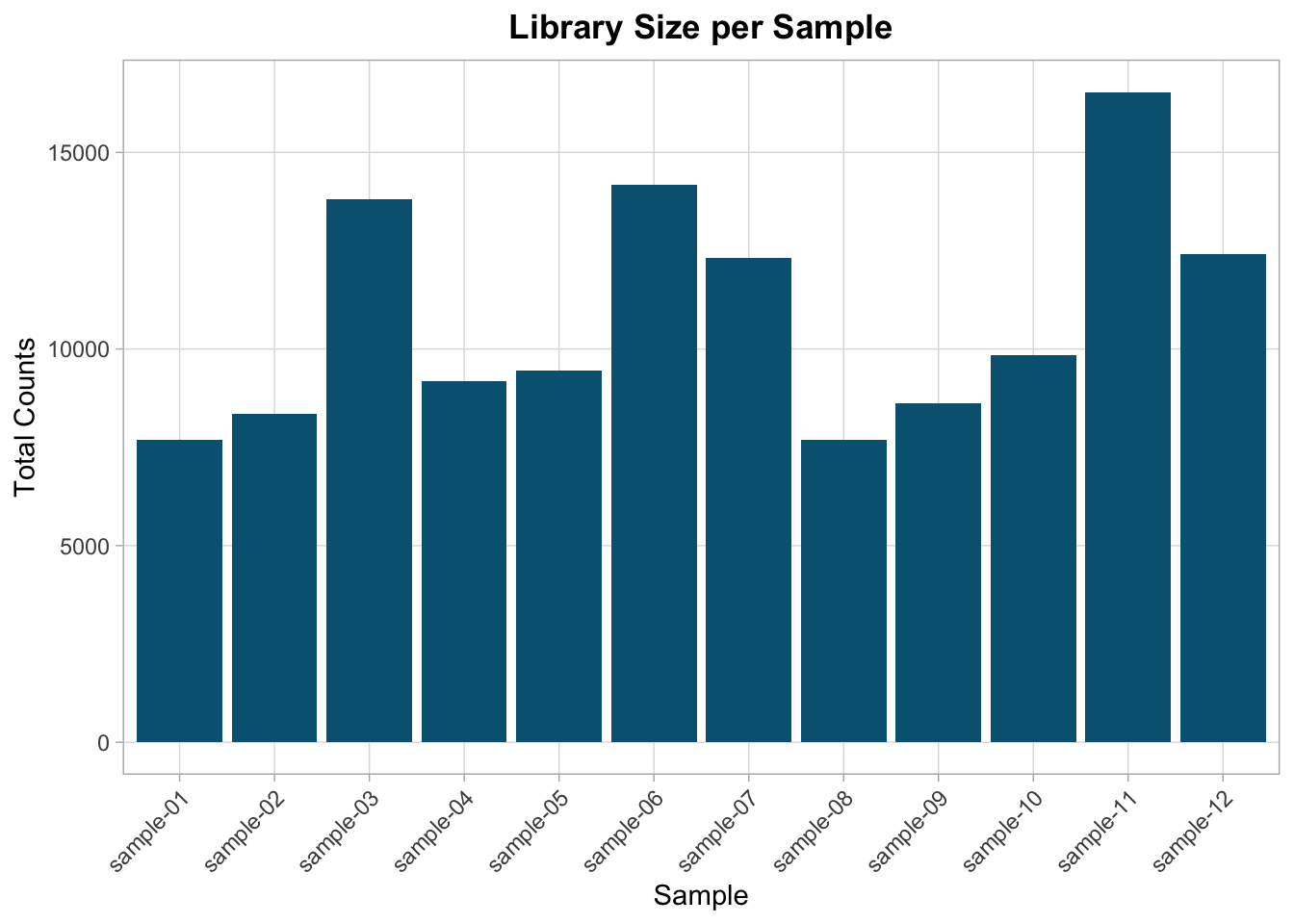
Moderate variation is expected.
Extreme outliers require investigation.
RNA-seq counts are typically right-skewed.
raw_values <- as.vector(as.matrix(counts[-1]))

ggplot2::ggplot(
  data.frame(count = raw_values),
  ggplot2::aes(x = count)
) +
  ggplot2::geom_histogram(bins = 50, fill = "#036281") +
  ggplot2::scale_x_continuous(trans = "log10") +
  ggplot2::labs(
    title = "Distribution of Raw Counts (log scale)",
    x = "Count (log10 scale)",
    y = "Frequency"
  ) +
  ggplot2::theme_light() +
  ggplot2::theme(
    plot.title = ggplot2::element_text(hjust = 0.5, face = "bold"),
    plot.subtitle = ggplot2::element_text(hjust = 0.5),
    panel.grid.minor = ggplot2::element_blank(),
    legend.position = "right"
  )
Warning in ggplot2::scale_x_continuous(trans = "log10"): log-10 transformation
introduced infinite values.Warning: Removed 108 rows containing non-finite outside the scale range
(`stat_bin()`).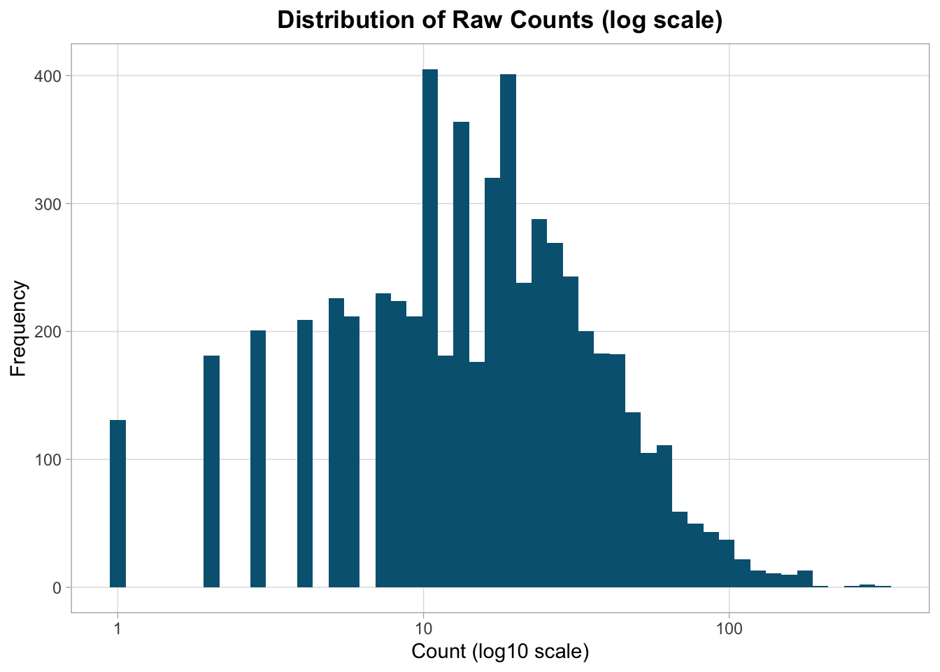
The heavy right tail reflects a small number of highly expressed genes.
log_counts <- log2(counts[-1] + 1)log_df <- tidyr::pivot_longer(
data.frame(sample = colnames(log_counts), t(log_counts)),
cols = -sample,
names_to = "gene",
values_to = "log_expression"
)
ggplot2::ggplot(log_df, ggplot2::aes(x = sample, y = log_expression)) +
ggplot2::geom_boxplot(fill = "#036281", outlier.size = 0.3) +
ggplot2::labs(
title = "Log2 Expression Distribution per Sample",
x = "Sample",
y = "Log2(count + 1)"
) +
ggplot2::theme_light() +
ggplot2::theme(
plot.title = ggplot2::element_text(hjust = 0.5, face = "bold"),
plot.subtitle = ggplot2::element_text(hjust = 0.5),
panel.grid.minor = ggplot2::element_blank(),
legend.position = "right",
axis.text.x = ggplot2::element_text(angle = 45, hjust = 1)
)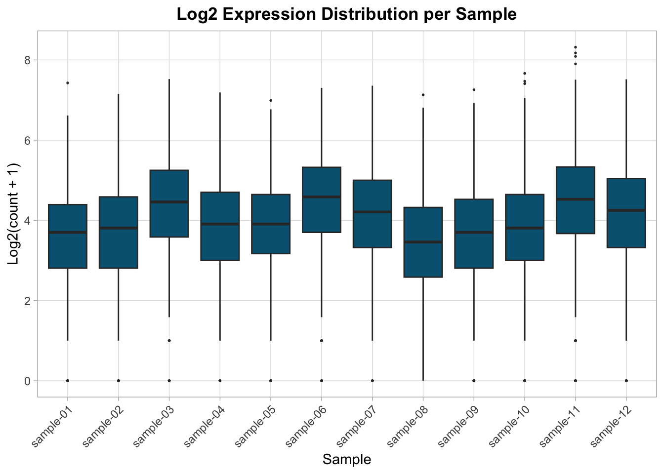
After log transformation, distributions should be more comparable.
Genes with extremely low counts across all samples contribute little information.
min_count_threshold <- 10

keep_genes <- rowSums(counts[-1] >= min_count_threshold) >= 3

sum(keep_genes)
[1] 430This keeps genes expressed at or above the threshold in at least three samples.
filtered_counts <- counts[keep_genes, ]

dim(filtered_counts)
[1] 430 13Filtering reduces noise and improves downstream stability.
Quality control at the count level ensures:
No modeling is performed yet.
We are preparing the matrix for meaningful normalization and exploratory analysis.